

In modern machine learning pipelines, predictive accuracy is frequently conflated with probabilistic reliability. When a classification algorithm outputs a probability score of 0.9 for a given instance, data scientists and automated decision systems routinely interpret this metric as a literal 90 percent confidence interval. However, empirical analysis often reveals a critical divergence: instances scored near 0.9 fail to achieve the anticipated positive outcome frequency. While the underlying model may rank instances effectively—distinguishing successfully between positive and negative classes—it frequently falters as an absolute arbiter of statistical certainty. This phenomenon, known as model miscalibration, presents profound risks in high-stakes domains such as clinical diagnostics, algorithmic credit scoring, and autonomous navigation, where uncalibrated confidence can precipitate systemic failure.
To address this systemic limitation in predictive modeling, developers rely on probability calibration techniques. Utilizing recent updates within the scikit-learn ecosystem—specifically the introduction of version 1.6 and its novel estimator management frameworks—practitioners can systematically diagnose and remediate probabilistic distortion. By implementing a rigorous methodology incorporating reliability diagrams, Brier scores, Platt scaling, and isotonic regression, machine learning engineers can bridge the gap between raw model scores and true statistical probabilities.
Understanding the Mechanics of Probability Calibration
A well-calibrated classifier is defined by its ability to yield prediction probabilities that directly correspond to empirical likelihoods. According to foundational machine learning evaluation standards, if a model groups a subset of samples into a probability bin centered around 0.8, approximately 80 percent of those specific samples must genuinely belong to the positive class. Standard performance metrics, including overall accuracy and the Area Under the Receiver Operating Characteristic Curve (ROC-AUC), are fundamentally incapable of verifying this criterion. Both metrics evaluate classification thresholds or ordinal rankings rather than absolute probabilistic alignment. Consequently, a model can achieve exceptional ROC-AUC scores while remaining severely overconfident or underconfident in its individual outputs.
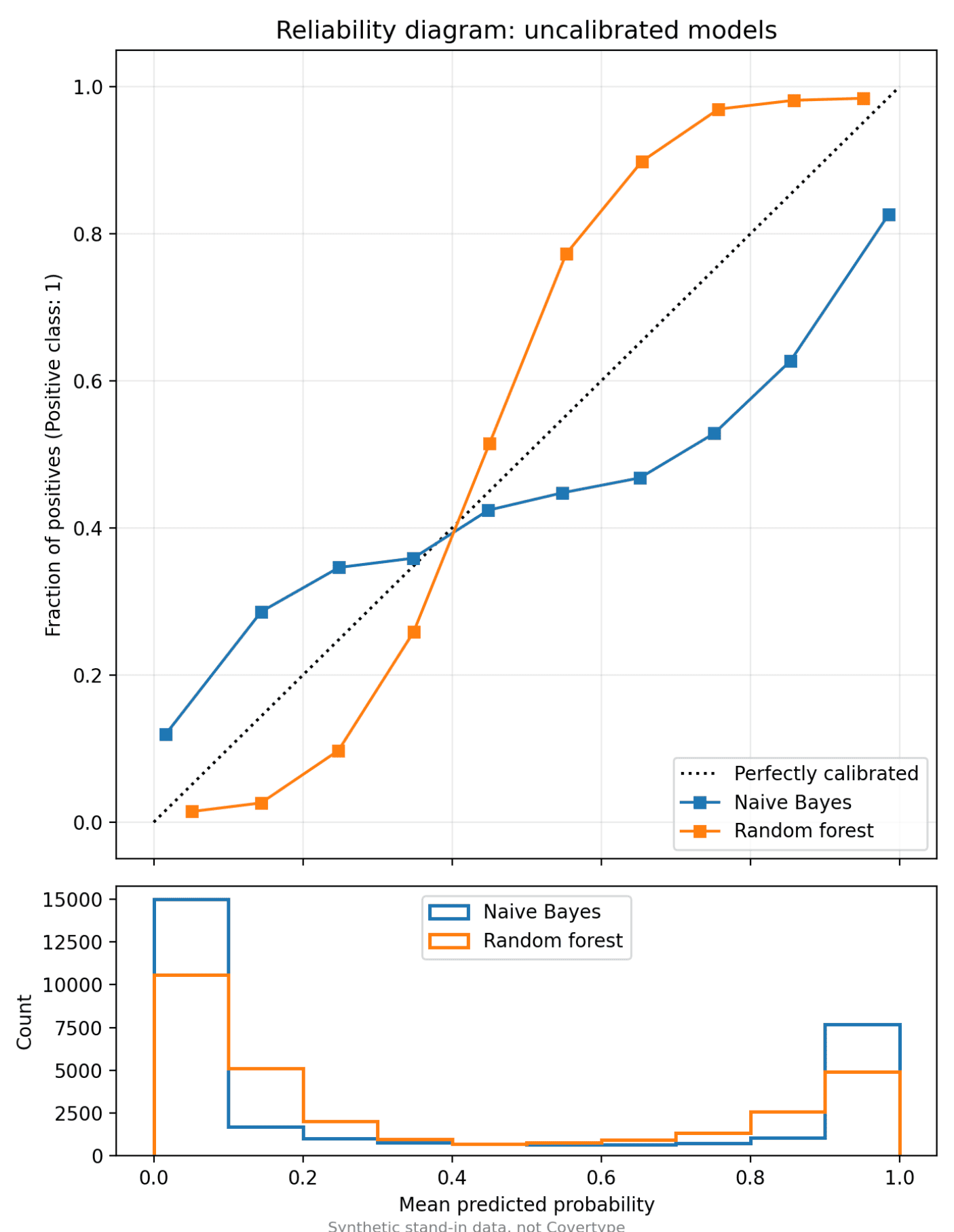
Different algorithmic architectures exhibit distinct propensities toward calibration failure. Logistic regression models, by virtue of their underlying loss function optimization, typically yield reliable probability estimates inherently. Conversely, Gaussian Naive Bayes classifiers notoriously push predicted probabilities toward the absolute boundaries of zero and one, driven by strict conditional independence assumptions that inflate confidence. Ensemble methods, such as random forests, tend to compress probabilities away from the extremes due to the averaging effects across numerous constituent decision trees. Meanwhile, maximum-margin classifiers like Support Vector Machines (SVMs) generate characteristic sigmoid-shaped distortions in their output distributions, necessitating external post-processing corrections.
Establishing the Experimental Environment and Dataset
To observe and correct these behaviors empirically, developers must configure a controlled testing environment using contemporary Python libraries. Proper execution requires scikit-learn version 1.6 or later, a release introducing significant architectural enhancements such as the FrozenEstimator class. This component deprecates legacy cross-validation configurations like cv="prefit", streamlining how pre-trained models interface with calibration wrappers.

The empirical analysis utilizes the widely benchmarked Forest Covertype dataset, accessible natively via scikit-learn. Originally curated for predicting dominant tree species across 581,012 cartographic grid cells characterized by 54 distinct physical features, the dataset provides a robust testing ground for binary classification tasks. By isolating a specific classification target—such as predicting Spruce/Fir occurrences against all alternative forest cover types—and downsampling the corpus to a manageable subset of 100,000 instances, engineers can execute rigorous computational experiments without sacrificing statistical validity.
Crucially, implementing robust probability calibration demands a strict three-way data partitioning strategy: training sets, calibration sets, and independent test sets. Machine learning models inherently exhibit higher confidence on data utilized during their training phase. Consequently, fitting a probability calibrator on training data results in learned probabilities that are artificially skewed toward extremes. To circumvent this bias, practitioners must train the base classifier on a dedicated training split, fit the calibration wrapper on an isolated validation subset, and reserve a strictly untouched test split for final performance evaluation.
import numpy as np
import matplotlib.pyplot as plt
from sklearn.calibration import CalibratedClassifierCV, CalibrationDisplay
from sklearn.datasets import fetch_covtype
from sklearn.ensemble import RandomForestClassifier
from sklearn.frozen import FrozenEstimator
from sklearn.metrics import brier_score_loss, log_loss, roc_auc_score
from sklearn.model_selection import train_test_split
from sklearn.naive_bayes import GaussianNB

RANDOM_STATE = 42

# Load and preprocess the Covertype dataset
X, y = fetch_covtype(return_X_y=True)
y = (y == 1).astype(int)  # Binary conversion: Spruce/Fir vs. Others

# Subsample to 100,000 records for computational efficiency
rng = np.random.default_rng(RANDOM_STATE)
subset = rng.choice(len(X), size=100_000, replace=False)
X, y = X[subset], y[subset]

# Partition into Train (50%), Calibration (20%), and Test (30%) sets
X_train, X_rest, y_train, y_rest = train_test_split(
    X, y, train_size=0.5, stratify=y, random_state=RANDOM_STATE
)
X_cal, X_test, y_cal, y_test = train_test_split(
    X_rest, y_rest, train_size=0.4, stratify=y_rest, random_state=RANDOM_STATE
)
Diagnosing Model Miscalibration
With the data partitioned, practitioners can train models known for contrasting calibration failures: a Gaussian Naive Bayes classifier and a Random Forest classifier. Following model fitting, diagnostic tools including Brier score losses, log losses, and reliability diagrams expose the extent of miscalibration.
The Brier score calculates the mean squared difference between predicted probabilities and the actual binary outcomes, where lower values indicate superior performance. However, because the Brier score simultaneously captures both calibration fidelity and discriminative capacity, it must be analyzed alongside visual reliability diagrams. These diagrams group predictions into discrete probability bins, plotting mean predicted probabilities against true empirical frequencies. A perfectly calibrated model aligns directly with the diagonal reference line, while deviations highlight systemic overconfidence or underconfidence.
Correcting Probabilities via Platt Scaling and Isotonic Regression
Once miscalibration is diagnosed, developers can apply post-processing correction algorithms via scikit-learn’s CalibratedClassifierCV. Two primary methodologies dominate the field: Platt scaling and isotonic regression.
Platt scaling applies a parametric logistic regression transformation to the outputs of the underlying model. Grounded in a sigmoid function governed by two parameters learned via maximum likelihood estimation, Platt scaling is exceptionally robust against overfitting. It is the preferred intervention when working with smaller calibration datasets or when preserving the exact ordinal ranking of predictions—and consequently the ROC-AUC score—is paramount. Furthermore, its parametric nature effectively models the sigmoid distortions typical of maximum-margin classifiers.
Alternatively, isotonic regression employs a non-parametric, piecewise constant monotonic function to remap predicted scores. Because it makes no structural assumptions regarding the underlying distribution shape, isotonic regression can correct complex, non-sigmoidal calibration curves. This flexibility, however, introduces vulnerability to overfitting when training data is scarce. Industry standards recommend reserving isotonic regression for calibration datasets exceeding one thousand instances, as smaller samples frequently trigger degraded generalization performance.
# Implementing Platt scaling and Isotonic regression calibration loops
calibrated_models =
for name, model in "Naive Bayes": GaussianNB(), "Random forest": RandomForestClassifier(n_estimators=200, random_state=RANDOM_STATE).items():
    for method in ("sigmoid", "isotonic"):
        calibrator = CalibratedClassifierCV(FrozenEstimator(model.fit(X_train, y_train)), method=method)
        calibrator.fit(X_cal, y_cal)
        calibrated_models[(name, method)] = calibrator.predict_proba(X_test)[:, 1]
Strategic Selection of Calibration Frameworks
Selecting the optimal calibration strategy requires careful alignment with operational constraints and dataset characteristics. When data availability is severely limited—falling below one thousand calibration samples—Platt scaling (method="sigmoid") remains the safest paradigm due to its constrained parameter space. Conversely, rich datasets comprising several thousand validation instances benefit from the expressive capacity of isotonic regression, provided that slight variations in ranking metrics are permissible.
For scenarios where reserving a dedicated validation split is infeasible, scikit-learn supports cross-validated calibration workflows. By instantiating CalibratedClassifierCV with an unfitted estimator and specifying a fold parameter (e.g., cv=5), the framework automatically orchestrates out-of-fold predictions. This ensures that the internal calibration algorithms evaluate exclusively on data unseen during the respective base model training phases, preventing data leakage.
Ultimately, integrating systematic probability calibration into machine learning pipelines transforms arbitrary numerical outputs into trustworthy confidence metrics. By acknowledging that predictive discrimination does not guarantee probabilistic accuracy, engineering teams can deploy automated systems that are not only precise in their decisions, but transparent and reliable in their stated certainties.
Related posts: